Bond Valuation

import numpy as np
import matplotlib.pyplot as plt
import scipy as sp
import pandas as pd
import datetime as dt
import numpy_financial as npf
import yfinance as yf
from scipy.optimize import minimize

plt.style.use("ggplot")

Here is a general logic of Bond Valuation: Adding up all present values of expected cash flows to equal the par value of the security.

Three procedures: 1. Estimate the cash flow (It’s simple if you hold treasury bills or bonds, because they are fixed. It’s way much more complicated for structured products like Mortgage-Backed Securities) 2. Which discount rate to use? (Require return = risk-free rate + risk premium) 3. Calculate the present values of all cash flows.

Zero Coupon Bond

Zero coupon bond returns you principal amount (face value) after certain period of time, no other cash payment is made.

The most common zero coupon bond is US treasury bill, you buy the bill with a discounted price, for instance the par value is \(\$1000\), you pay \(\$950\) today and receives the par value \(\$1000\) one year later.

In reality, treasury bills has different maturities, such as 4 week, 8 weeks or the longest 52 weeks.

class ZeroCouponBonds:

    def __init__(self, principal, maturity, discount_rate):
        self.principal = principal
        self.maturity = maturity  # date to maturity
        self.discount_rate = discount_rate  # risk-free interest rate

    def calculate_pv(self):
        return self.principal / (1 + self.discount_rate) ** self.maturity

bond = ZeroCouponBonds(1000, 3, 0.04)

bond.calculate_pv()

888.9963586709148

discount_rate_array = np.linspace(0.01, 0.1)
pv_array = []
for i in discount_rate_array:
    pv_array.append(ZeroCouponBonds(1000, 3, i).calculate_pv())

fig, ax = plt.subplots(figsize=(12, 6))
ax.plot(discount_rate_array, pv_array)
ax.set_title("$\$1000$ zero-coupon bond price")
ax.set_xlabel("discount rate")
plt.show()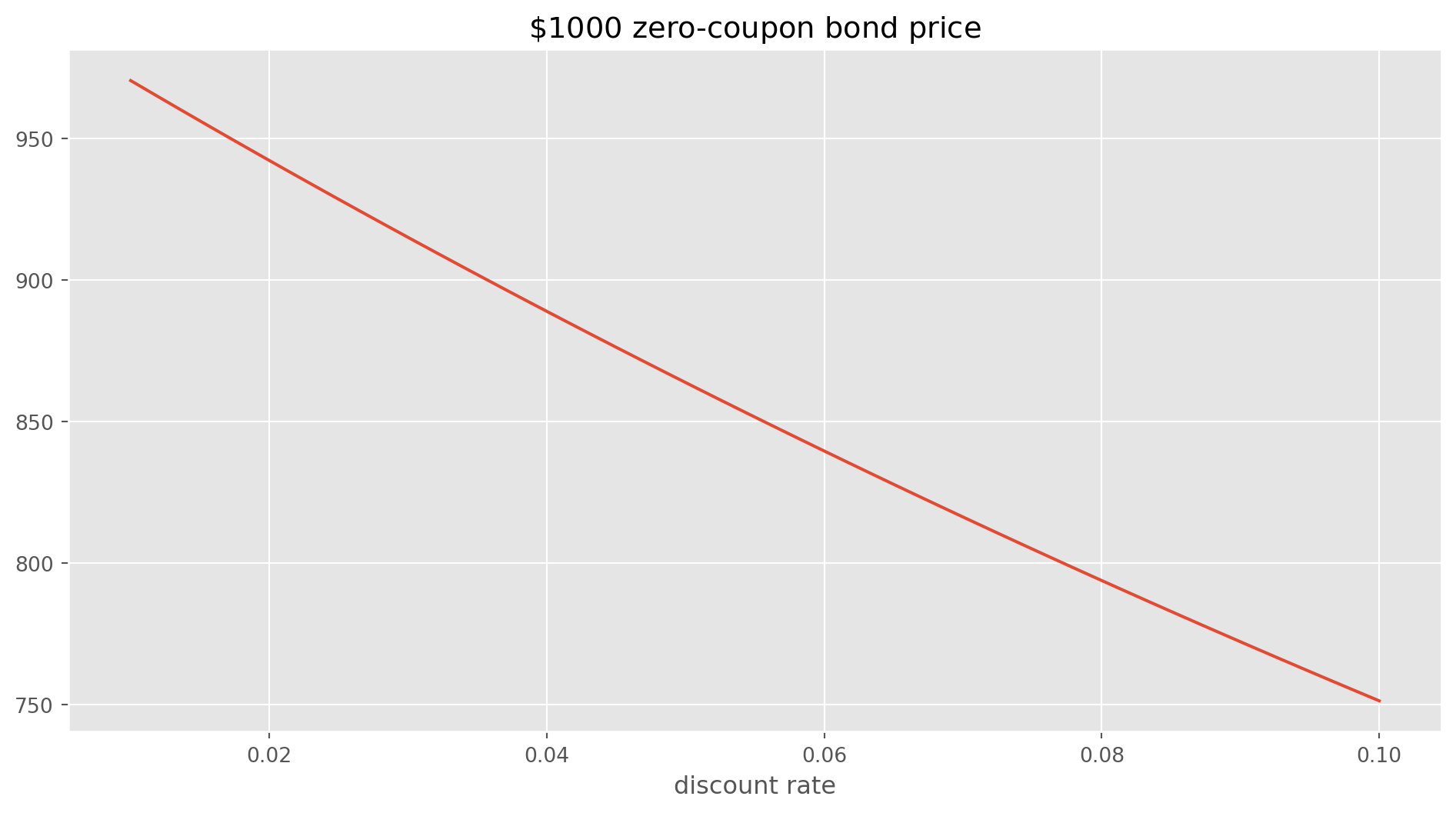

Coupon Bond

Coupon bonds are the one paying regular coupons till maturity. The pricing formula is

\[ P= \sum_{t=1}^n \frac{C_t}{(1+r)^t}+\frac{B}{(1+r)^n} \]

where \(C\) is coupon, B is the par value, n is the maturity.

3 year maturity, coupon rate \(10\%\), annual payment, par value \(\$1000\), discount rate (YTM) is \(4\%\).

class CouponBond:

    def __init__(self, principal, coupon_rate, maturity, discount_rate):
        self.principal = principal
        self.coupon_rate = coupon_rate
        self.maturity = maturity
        self.discount_rate = discount_rate

    def calculate_pv(self, x, n):
        return x / (1 + self.discount_rate) ** n

    def calculate_bond_price(self):
        price = 0
        for t in range(1, self.maturity + 1):
            price = price + self.calculate_pv(self.principal * self.coupon_rate, t)
        price = price + self.calculate_pv(self.principal, self.maturity)
        return price

bond = CouponBond(1000, 0.1, 3, 0.08)

bond.calculate_bond_price()

1051.5419397449573

discount_rate_array = np.linspace(0.01, 0.15)
pv_array = []
for i in discount_rate_array:
    pv_array.append(CouponBond(1000, 0.1, 3, i).calculate_bond_price())

fig, ax = plt.subplots(figsize=(12, 6))
ax.plot(discount_rate_array, pv_array)
ax.set_title("$\$1000$ coupon bond price")
ax.set_xlabel("discount rate")
ax.scatter(0.1, 1000, s=100)
plt.show()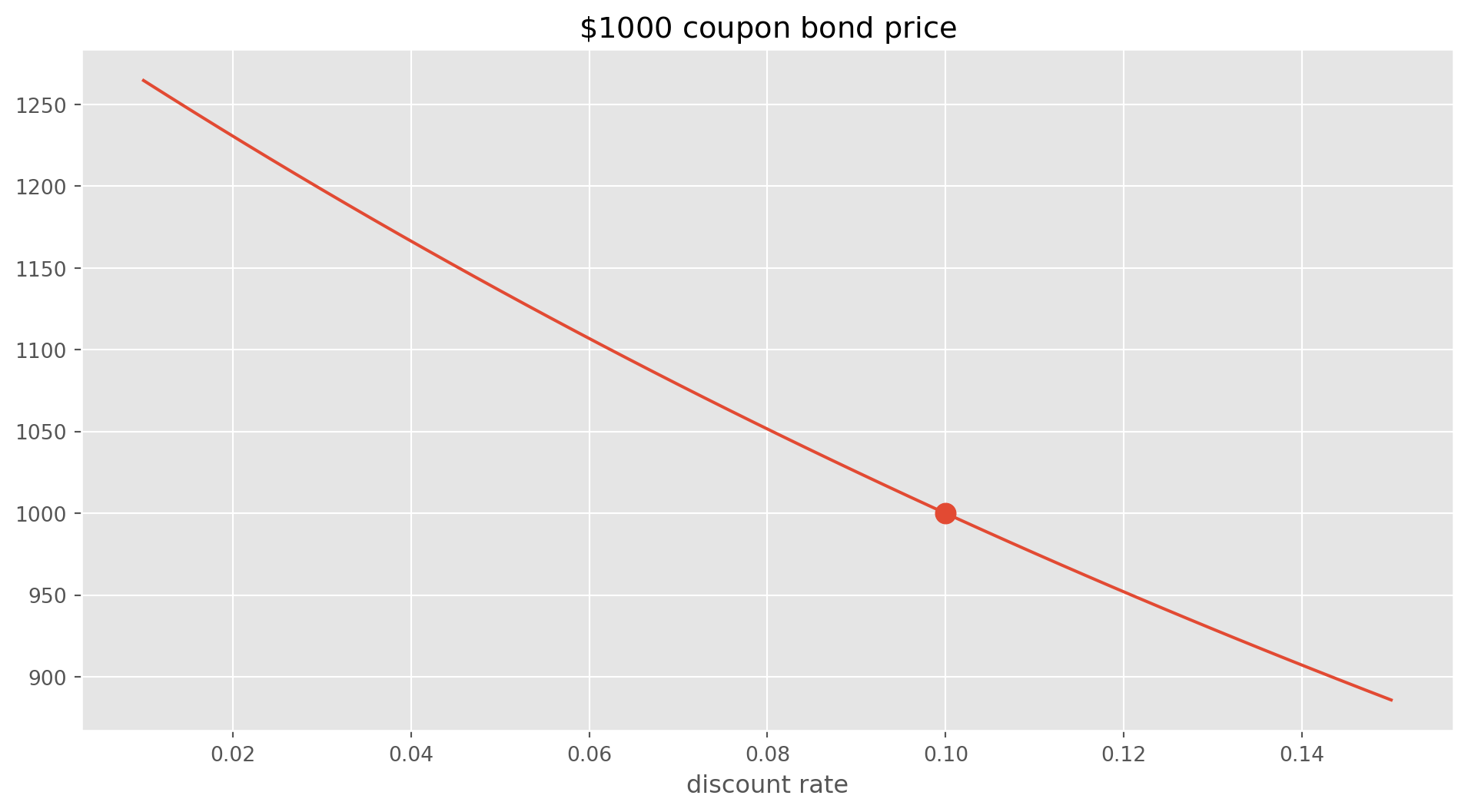

From the chart, we know that if discount rate equals coupon rate, in this case \(10\%\), it’s called par bond. If the price is larger than face value, it is premium bond, vice verse discount bond.

Portfolio Management

If you are not a single asset trader, you will end up constructing your portfolio sooner or later. In the view of portfolio management, the risk of single type of asset is not a major concern anymore, rather the risk of portfolio, e.g. you might need to consider have derivatives in your portfolios too.

1. Planning

• State your investment objectives and constraints. (Institutions usually use Investment Policy Statement)
  
• Review your objective benchmark regularly
  

2. Execution

• Asset allocation
  
• Security Analysis
  
• Portfolio construction
  

3. Feedback

• Monitor and rebalance portfolio
  
• Measure portfolio performance
  

Performance Measuring

Two methods of measuring portfolio’s performance.

Time-Weight Rate of Return

Basically it’s annualized geometric mean.

Suppose you hold a portfolio for 3 years, at the end of first year the return is 12%, second year 2%, third year 7%.

The geometric mean function can return a TWRR directly, if the holding period is long than 1 year.

sp.stats.gmean([12, 2, 7])

5.517848352762241

Now suppose you hold a portfolio for 1 year, at the end of first season the return is 1%, the second season 4%, the third season -5%, the forth season 8%.

np.prod([1.01, 1.04, 0.95, 1.08]) - 1

0.07771039999999996

The general formula is \[ \text{TWRR} = \left[\prod_{i=1}^N(1+\text{HPR}_i)\right]^{1/n}-1 \]

TWRR measures the compound rate of return, where \(n\) is number of years, \(N\) the number of periods, \(\text{HPR}\) means holding period return.

As a reminder, for audiences familiar with another measurement Compound Annual Growth Rate \(\text{CAGR}\) \[ C A G R=\left[\left(\frac{E V}{B V}\right)^{1/n}-1\right]\times 100 \] where: \(E V=\) Ending value
\(B V=\) Beginning value
\(n=\) Number of years

Both are geometric means, but \(\text{TWRR}\) measures returns of every period.

Example of TWRR

You bought a share of a mutual fund for \(\$100\) at \(t=0\), another share at \(\$113\) at \(t=1\), also you receive dividend \(\$4\) at \(t=1\), \(\$7\) at \(t=2\) per share.Then you redeem both shares for \(\$120\) at \(t=2\).

Calculate TWRR.

fund = {"price": [100, 113, 120], "dividend": [0, 4, 7]}
fund = pd.DataFrame(fund)
fund

	price	dividend
0	100	0
1	113	4
2	120	7

HPR_1 = (113 + 4) / 100 - 1
HPR_2 = (120 * 2 + 7 * 2) / (113 * 2) - 1

np.sqrt((1 + HPR_1) * (1 + HPR_2)) - 1

0.14671520100345292

Money-Weight Rate of Return

Basically annualized IRR.

Example of MWRR

You bought a share of a mutual fund for \(\$100\) at \(t=0\), another share at \(\$113\) at \(t=1\), also you receive dividend \(\$4\) at \(t=1\), \(\$7\) at \(t=2\) per share.Then you redeem both shares for \(\$120\) at \(t=2\).

Calculate MWRR.

The key of MWRR is to identify net cash flow for each period, then calculate IRR.

npf.irr([-100, -113 + 4, 120 * 2 + 7 * 2])

0.1393470544991613

To summarize, MWRR takes account of cash flow, TWRR does not.

Modern Portfolio Theory

MPT states that investors can construct optimal portfolios offering maximum possible expected return for a given risk level.

Assumption: 1. Return of assets are normally distributed. 2. Investors are risk-averse. (Higher return, higher risks.) 3. Investors are only long positions only.

Efficiency Frontier

Definition of Portfolio Return and Volatility

Commonly the MPT is illustrated by matrices. Define \(\mathbf{R}\) and \(\mathbf{w}\)

\[ \mathbf{R}=\left[\begin{array}{c} R_1 \\ R_2 \\ R_3 \end{array}\right], \quad \mathbf{w}=\left[\begin{array}{l} w_1 \\ w_2 \\ w_3 \end{array}\right] \] where \(R_i\) represents the return of asset \(i\); \(w_i\) the weight of asset \(i\)

The expected return and covariance matrix of return is \[ E[\mathbf{R}]=\left[\begin{array}{l} E\left[R_1\right] \\ E\left[R_2\right] \\ E\left[R_3\right] \end{array}\right]=\left[\begin{array}{c} \mu_1 \\ \mu_2 \\ \mu_3 \end{array}\right]=\boldsymbol{\mu} \]

\[ \begin{aligned} \operatorname{var}(\mathbf{R}) & =\left[\begin{array}{ccc} \operatorname{var}\left(R_1\right) & \operatorname{cov}\left(R_1, R_2\right) & \operatorname{cov}\left(R_1, R_3\right) \\ \operatorname{cov}\left(R_2, R_1\right) & \operatorname{var}\left(R_2\right) & \operatorname{cov}\left(R_2, R_3\right) \\ \operatorname{cov}\left(R_3, R_1\right) & \operatorname{cov}\left(R_3, R_2\right) & \operatorname{var}\left(R_3\right) \end{array}\right] \\ & =\left[\begin{array}{ccc} \sigma_1^2 & \sigma_{1, 2} & \sigma_{1, 3} \\ \sigma_{1,2} & \sigma_2^2 & \sigma_{2,3} \\ \sigma_{1,3} & \sigma_{2,3} & \sigma_3^2 \end{array}\right]=\mathbf{\Sigma} \end{aligned} \]

The portfolio return is obtained by inner product of \(\mathbf{w}\) and \(\mathbf{R}\)

\[ R_{p}=\mathbf{x}^{T} \mathbf{R}=\left[w_1, w_2, w_3\right]\left[\begin{array}{c} R_A \\ R_B \\ R_C \end{array}\right]=x_1 R_1+x_2 R_2+x_3 R_3 \] where \(R_p\) represents portfolio return. Similarly, the expected portfolio return is \[ w_1 \mu_1+w_2 \mu_2+w_3 \mu_3 \]

The variance of the portfolio is \[ \sigma_{p}^2=\operatorname{var}\left[\mathbf{w}^{T} \mathbf{R}\right]=\mathbf{w}^{T} \Sigma \mathbf{w}=\left[x_1, x_2, x_3\right]\left[\begin{array}{ccc} \sigma_1^2 & \sigma_{1,2} & \sigma_{1,3} \\ \sigma_{1,2} & \sigma_2^2 & \sigma_{2,3} \\ \sigma_{1,3} & \sigma_{2,3} & \sigma_3^2 \end{array}\right]\left[\begin{array}{l} x_1 \\ x_2 \\ x_3 \end{array}\right] \]

This is a standard quadratic form, for more details, check quadratic form and multivariate normal distribution.

Sharpe Ratio

Sharpe Ratio \[SR=\frac{R_p-R_f}{\sigma_p}\] where: \(R_p=\) return of portfolio
\(R_f=\) risk-free rate
\(\sigma_p=\) standard deviation of the portfolio’s excess return

Retrieve Data

stocks = ["AMZN", "HD", "MRNA", "TSLA", "LULU"]
start_date = "2015-01-01"
end_date = dt.datetime.today()

def download_data(stocks, dropna):
    # dropna decides if you want to drop all NaN values
    stock_data = {}
    for stock in stocks:
        ticker = yf.Ticker(stock)
        stock_data[stock] = ticker.history(start=start_date, end=end_date)["Close"]
    if dropna == True:
        df = pd.DataFrame(stock_data).dropna()
    else:
        df = pd.DataFrame(stock_data)
    return df

df = download_data(stocks, dropna=True)
df.head()

	AMZN	HD	MRNA	TSLA	LULU
Date
2018-12-07 00:00:00-05:00	81.456497	147.259521	18.600000	23.864668	113.870003
2018-12-10 00:00:00-05:00	82.051498	146.322021	18.799999	24.343332	115.010002
2018-12-11 00:00:00-05:00	82.162003	146.765259	18.010000	24.450666	116.849998
2018-12-12 00:00:00-05:00	83.177002	148.469711	18.680000	24.440001	122.650002
2018-12-13 00:00:00-05:00	82.918999	148.179932	18.760000	25.119333	120.199997

def plot_data(size, data, title):
    # choose the size of the figure [w, h]
    data.plot(figsize=(size[0], size[1]), title=title)
    plt.show()

plot_data([12, 6], df, title="Close Price Plot")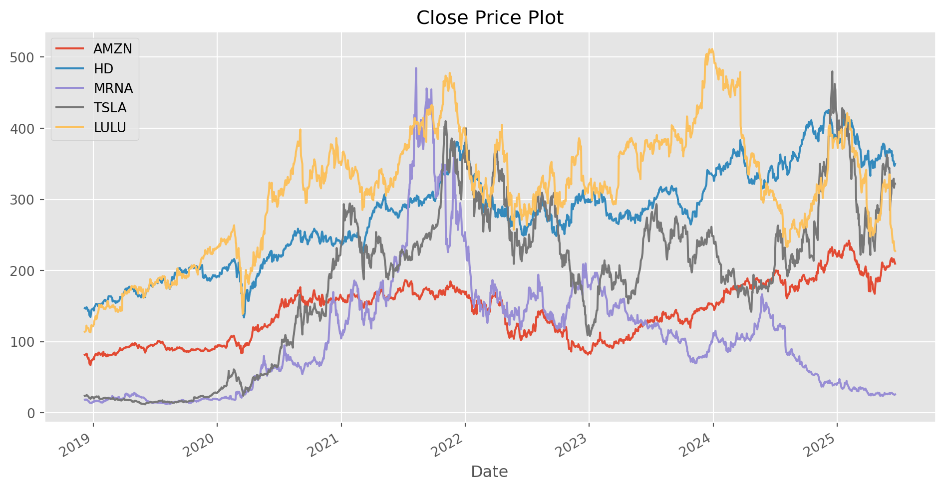

def cal_log_return(data):
    return (np.log(data) - np.log(data.shift())).dropna()

log_ret_daily = cal_log_return(df)

plot_data([12, 6], log_ret_daily, title="Log Return Plot")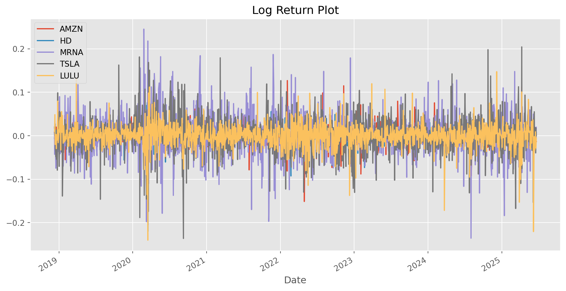

Calculate Expected Return and Volatility

# assume the average trading days in a year is 252
num_trading_days = 252

def cal_statistics(returns):
    # mean of annual return
    print(returns.mean() * num_trading_days)

cal_statistics(log_ret_daily)

AMZN    0.145205
HD      0.132780
MRNA    0.050842
TSLA    0.399676
LULU    0.106261
dtype: float64

weights = np.array([0.2, 0.1, 0.4, 0.1, 0.1])

\[ \mu = \sum_i w_i \mu_i \] where \(\mu\) is expected portfolio return, \(w\) is the weight, \(\mu_i\) is the expected rate of return on a specific asset.

\[ \mathbf{w}^{T} \Sigma \mathbf{w} \]

def show_mean_var(returns, weights):
    portfolio_return = np.sum(returns.mean() * weights) * num_trading_days
    portfolio_volatility = np.dot(
        weights.T, np.dot(returns.cov() * num_trading_days, weights)
    )
    print("portfolio return: {}".format(portfolio_return))
    print("portfolio volatility: {}".format(portfolio_volatility))
    return portfolio_return, portfolio_volatility

show_mean_var(log_ret_daily, weights)

portfolio return: 0.11324963347558487
portfolio volatility: 0.1275179090538697

(0.11324963347558487, 0.1275179090538697)

Simulate Portfolios

num_portfolio = 5000


def gen_portfolio(returns, stocks):

    portfolio_weights = []
    portfolio_means = []
    portfolio_volatilities = []

    for i in range(num_portfolio):
        w = np.random.rand(len(stocks))
        w = w / np.sum(w)
        portfolio_weights.append(w)
        portfolio_means.append(np.sum(returns.mean() * w) * num_trading_days)
        portfolio_volatilities.append(
            np.sqrt(np.dot(w.T, np.dot(returns.cov() * num_trading_days, w)))
        )
    return (
        np.array(portfolio_weights),
        np.array(portfolio_means),
        np.array(portfolio_volatilities),
    )

portfolio_weights, portfolio_means, portfolio_volatilities = gen_portfolio(
    log_ret_daily, stocks
)

plt.rcParams["axes.grid"] = (
    False  # this is unnecessary, but without it, a bug warning will be triggered
)


def portfolio_scatter(returns, volatilities):
    fig, ax = plt.subplots(figsize=(12, 6))
    mpt = ax.scatter(
        volatilities, returns, c=returns / volatilities
    )  # actually we didn't use risk-free rate as reference for SR
    ax.set_xlabel("Expected Volatilities")
    ax.set_ylabel("Expected Returns")
    ax.grid()
    fig.colorbar(mpt, label="Sharpe Ratio")
    plt.show()

portfolio_scatter(portfolio_means, portfolio_volatilities)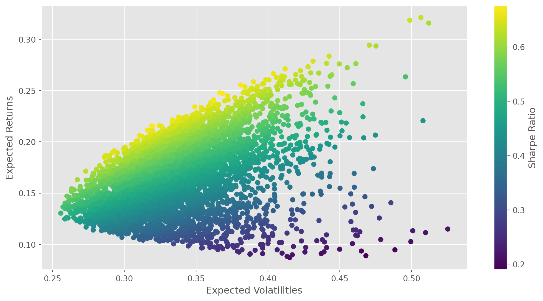

Global Minimum Variance Portfolio

For demonstrating purpose, denote the weight of global minimum variance of \(n\) assets portfolio as \(\mathbf{w}_g=(w_{1,g},w_{2,g},w_{3,g}, ..., w_{n,g})\)

\[ \begin{gathered} \min _{\mathbf{w}} \mathbf{w}^{T} \Sigma \mathbf{w}\\ \text { s.t. } \sum_{i=1}^n w_{i,g}=1 \end{gathered} \]

You can obtain F.O.C by performing partial derivative on the Lagrangian form, however it can be absurdly tedious, therefore we skill this step.

In short, to arrange the F.O.C. in matrix form, we obtain \[ \left[\begin{array}{cc} 2 \boldsymbol{\Sigma} & \mathbf{1} \\ \mathbf{1}^{T} & 0 \end{array}\right]\left[\begin{array}{c} \mathbf{w} \\ \lambda \end{array}\right]=\left[\begin{array}{l} \mathbf{0} \\ 1 \end{array}\right] \]

where \(\boldsymbol{\Sigma}\) is covariance matrix, \(\mathbf{1}\) and \(\mathbf{0}\) is a \(n-1\) vector of \(1\)’s and \(0\)’s.

The solution is straightforward in linear algebra form

\[ \left[\begin{array}{c} \mathbf{w} \\ \lambda \end{array}\right]=\left[\begin{array}{cc} 2 \boldsymbol{\Sigma} & \mathbf{1} \\ \mathbf{1}^{T} & 0 \end{array}\right]^{-1}\left[\begin{array}{l} \mathbf{0} \\ 1 \end{array}\right] \]

Efficient Portfolio

The formulation of portfolio optimization follows a standard microeconomic optimization duality, i.e. maximize the expected return subject to a certain risk, or minimize the risk subject to a certain rate of expected rate.

\[ \begin{aligned} \max _{\mathbf{x}} \mu_p & =\mathbf{w}^{T} \boldsymbol{\mu} \\ \text { s.t. }\mathbf{w}^{T} \boldsymbol{\Sigma} \mathbf{w}&=\sigma_{p, 0}^2 \text { and } \mathbf{w}^{T} \mathbf{1}=1 \end{aligned} \]

\[ \begin{aligned} \min _{\mathbf{w}} \sigma_{p, w}^2 & =\mathbf{w}^{T} \boldsymbol{\Sigma} \mathbf{w} \\ \text { s.t. }\mathbf{w}^{T} \boldsymbol{\mu}&=\mu_{p, 0}, \text { and } \mathbf{w}^{T} \mathbf{1}=1 \end{aligned} \]

where \(\sigma_{p,0}^2\) is the target portfolio variance and \(\mu_{p, 0}\) is the target portfolio expected return.

Theoretically, you can pick any formulation you like, but in practice the latter is more common due to its computational convenience.

The efficient frontier is a graph of \(\mu_p\) and \(\sigma_p\) resembles one side of hyperbola as we have shown above, and is often called the ‘Markowitz Bullet’.

Two constraints for two \(\lambda\)’s, the Lagrangian formulation is \[ L\left(\mathbf{w}, \lambda_1, \lambda_2\right)=\mathbf{w}^{T} \boldsymbol{\Sigma} \mathbf{w}+\lambda_1\left(\mathbf{w}^{T} \boldsymbol{\mu}-\mu_{p, 0}\right)+\lambda_2\left(\mathbf{w}^{T} \mathbf{1}-1\right) \]

The F.O.C.s for a minimum are \[ \begin{aligned} & \frac{\partial L\left(\mathbf{w}, \lambda_1, \lambda_2\right)}{\partial \mathbf{w}}=2 \boldsymbol{\Sigma} \mathbf{w}+\lambda_1 \boldsymbol{\mu}+\lambda_2 \mathbf{1}=\mathbf{0} \\ & \frac{\partial L\left(\mathbf{w}, \lambda_1, \lambda_2\right)}{\partial \lambda_1}=\mathbf{w}^{T} \boldsymbol{\mu}-\mu_{p, 0}=0 \\ & \frac{\partial L\left(\mathbf{w}, \lambda_1, \lambda_2\right)}{\partial \lambda_2}=\mathbf{w}^{T} \mathbf{1}-1=0 . \end{aligned} \]

We can represent the system of linear equations using matrix as \[ \left(\begin{array}{ccc} 2 \boldsymbol{\Sigma} & \boldsymbol{\mu} & \mathbf{1} \\ \boldsymbol{\mu}^{\prime} & 0 & 0 \\ \mathbf{1}^{\prime} & 0 & 0 \end{array}\right)\left(\begin{array}{c} \mathbf{w} \\ \lambda_1 \\ \lambda_2 \end{array}\right)=\left(\begin{array}{c} \mathbf{0} \\ \mu_{p, 0} \\ 1 \end{array}\right) \] or \[ \mathbf{A} \mathbf{z}_w=\mathbf{b}_0, \] where \[ \mathbf{A}=\left(\begin{array}{ccc} 2 \boldsymbol{\Sigma} & \boldsymbol{\mu} & \mathbf{1} \\ \boldsymbol{\mu}^{T} & 0 & 0 \\ \mathbf{1}^{T} & 0 & 0 \end{array}\right), \mathbf{z}_w=\left(\begin{array}{c} \mathbf{w} \\ \lambda_1 \\ \lambda_2 \end{array}\right) \text { and } \mathbf{b}_0=\left(\begin{array}{c} \mathbf{0} \\ \mu_{p, 0} \\ 1 \end{array}\right) \] The solution for \(\mathbf{z}_w\) is then \[ \mathbf{z}_w=\mathbf{A}^{-1} \mathbf{b}_0 \]

Optimization Algorithm

def statistics(weights, returns):
    portfolio_returns = np.sum(returns.mean() * weights) * num_trading_days
    portfolio_volatilities = np.sqrt(
        np.dot(weights, np.dot(returns.cov() * num_trading_days, weights))
    )
    portfolio_sharpe_ratio = portfolio_returns / portfolio_volatilities
    return portfolio_returns, portfolio_volatilities, portfolio_sharpe_ratio

In practice, we could also minimize the negative Sharpe ratio, because \(\text{max} f(x) = \text{min} [-f(x)]\)

def neg_sharpe(weights, returns):
    return -statistics(weights, returns)[2]  # this is the negative sharpe ratio

Here we use lambda function, as a reminder of expression format \[ \text{lambda arguments : expression} \]

def optimize_portfolio(weights, log_returns):
    constraints = {"type": "eq", "fun": lambda x: np.sum(x) - 1}
    bounds = tuple((0, 1) for i in range(len(stocks)))
    return minimize(
        fun=neg_sharpe,
        x0=weights[0],
        args=log_returns,
        method="SLSQP",
        bounds=bounds,
        constraints=constraints,
    )

def print_optimal_portfolio(optimum, returns):
    print(
        "Optimal portfolio: ", optimum["x"].round(3)
    )  # 'x' is the solution array of OptimizeResult object
    print(
        "Expected return, volatility and SR: ",
        statistics(optimum["x"].round(3), returns),
    )

def plot_optimal_portfolio(optimal, returns, portfolio_returns, portfolio_volatility):
    figure, ax = plt.subplots(figsize=(12, 6))
    ax.scatter(
        portfolio_volatility,
        portfolio_returns,
        c=portfolio_returns / portfolio_volatility,
    )
    ax.scatter(
        statistics(optimal["x"], returns)[1],
        statistics(optimal["x"], returns)[0],
        s=100,
        marker=(5, 1),
    )
    ax.set_xlabel("Expected Volatility")
    ax.set_ylabel("Expected Returns")
    plt.show()

optimum = optimize_portfolio(portfolio_weights, log_ret_daily)
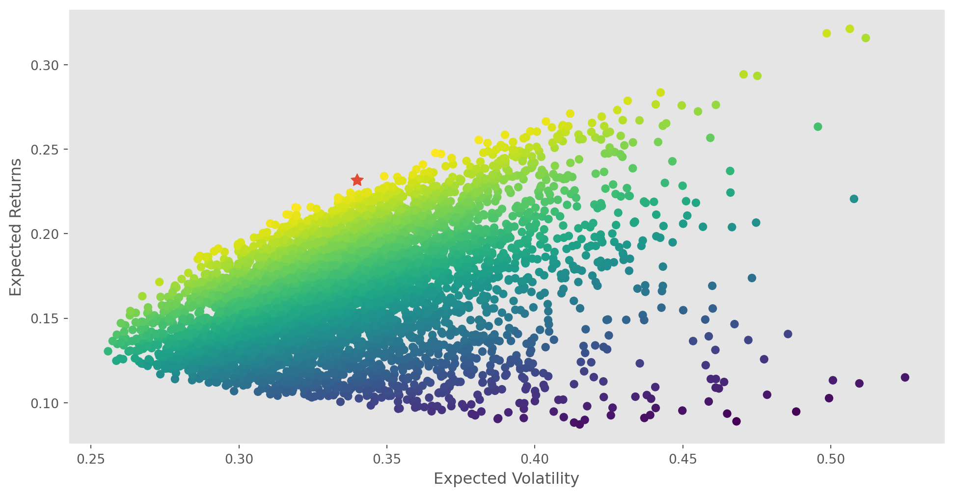
print_optimal_portfolio(optimum, log_ret_daily)

Optimal portfolio:  [0.11  0.524 0.    0.366 0.   ]
Expected return, volatility and SR:  (0.23183050271279573, 0.3400163438588997, 0.6818216444589528)

plot_optimal_portfolio(optimum, log_ret_daily, portfolio_means, portfolio_volatilities)